18: Iron — Berry curvature, anomalous Hall conductivity and optical conductivity

• Outline: Calculate the Berry curvature, anomalous Hall conductivity, and (magneto)optical conductivity of ferromagnetic bcc Fe with spin-orbit coupling. In preparation for this example it may be useful to read Ref. ¹ and Ch. 11 of the User Guide.

1-6. Compute the MLWFs and compute the energy eigenvalues and spin expectation values.

These are the same six steps of Tutorial solution 17 and therefore the results are not going to be showed here again.

Berry curvature plots

The Berry curvature \(\Omega_{\alpha\beta}(\mathbf{k})\) of the occupied states is defined in Eq. (11.18) of the User Guide. Plot the Berry curvature component \(\Omega_z(\mathbf{k}) = \Omega_{xy}(\mathbf{k})\) along the magnetization direction.

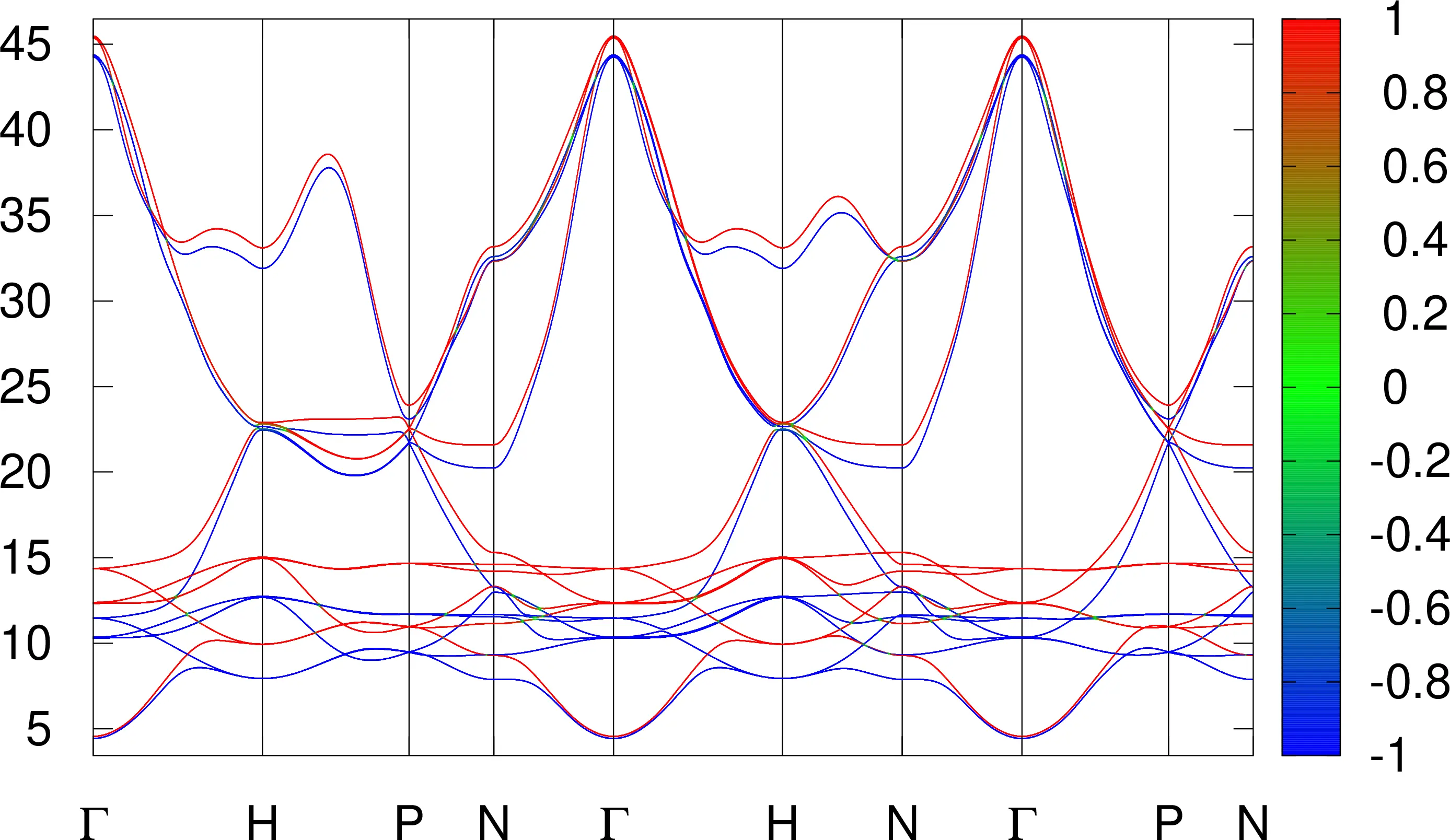
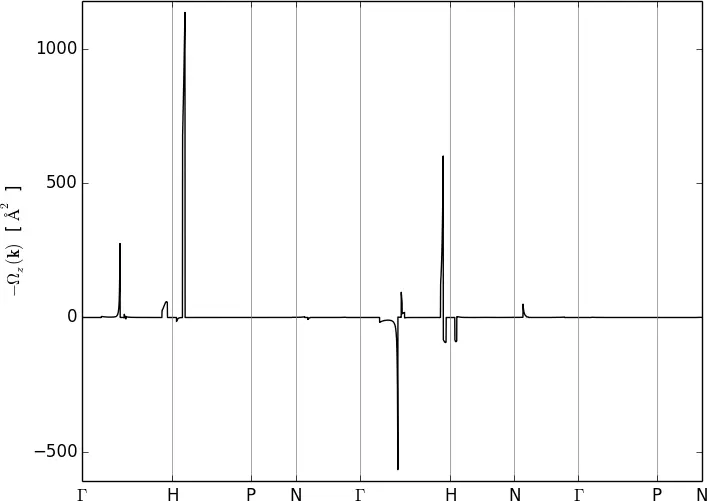
The Fermi energy should be \(12.6283\) eV. With this value we obtain the energy bands and the Berry curvature component \(\Omega_z(\mathbf{k}) = \Omega_{xy}(\mathbf{k})\) along high-symmetry points shown in Figure 1 and Figure 2. Eq. (11.18) of the User Guide is reported below for completeness.

\[\Omega_{\alpha\beta}(\mathbf{k}) = \sum_{n}^{occ} f_{n\mathbf{k}}\Omega_{n,\alpha\beta},\]

with

\[\Omega_{n,\alpha\beta} = \varepsilon_{\alpha\beta\gamma}\Omega_{n,\gamma} = -2\;\mathrm{Im}\langle \nabla_{k_\alpha}u_{n\mathbf{k}} \vert \nabla_{k_\beta}u_{n\mathbf{k}} \rangle,\]

where the Greek letters indicate Cartesian coordinates, \(\varepsilon_{\alpha\beta\gamma}\) is the Levi-Civita antisymmetric tensor, and \(\vert u_{n\mathbf{k}}\rangle\)s are the cell-periodic Bloch functions.

Band structure of Fe along symmetry lines Γ-H-P-N-Γ-H-N-Γ-P-N.

Berry curvature \(\Omega_z(\mathbf{k})\) in Fe along symmetry lines.

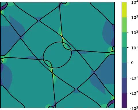
Combine the plot of the Fermi lines on the \(k_y\) plane with a heat-map plot of (minus) the Berry curvature.

The plot of the Fermi lines with a colour-map of \(-\Omega_z(k_x,0,k_z)\) is shown in Figure 3.

(Colour online) Calculated total Berry curvature \(-\Omega_z(\mathbf{k})\) in the plane \(k_y=0\) (note log scale). Intersections of the Fermi surface with this plane are shown.

Anomalous Hall conductivity

AHC converges rather slowly with k-point sampling, and a \(25 \times 25 \times 25\) does not yield a well-converged value. Compare the converged AHC value with those obtained in Refs. ² and ¹.

The x,y,z-components of the AHC for a \(25\times25\times25\) BZ mesh are shown in the snippet below. The converged result reported in Refs. ² and ¹ for the z-component is 756.76 (\((\Omega \mathrm{cm})^{-1}\)). Hence, a \(25\times25\times25\) BZ mesh clearly gives a very inaccurate value (\(\sim 36.4\%\) error). Even with adaptive refinement the error is still very large (\(\sim 31.7\%\)). It is worth to note that the adaptive refinement slightly breaks the symmetry and gives non-zero values for the x-component and y-component, although these are opposite in sign.

Without adaptive refinement

 Properties calculated in module  b e r r y
 ------------------------------------------

   * Anomalous Hall conductivity

 Interpolation grid: 25 25 25

 Fermi energy (ev):   12.6283

 AHC (S/cm)       x          y          z
 ==========    -0.0000     0.0000   554.6437

 Total Execution Time          59.112 (sec)

With adaptive refinement

 Properties calculated in module  b e r r y
 ------------------------------------------

   * Anomalous Hall conductivity

 Regular interpolation grid: 25 25 25
   Adaptive refinement grid: 5 5 5
       Refinement threshold: Berry curvature >100.00 bohr^2
  Points triggering refinement:   42( 0.27%)

 Fermi energy (ev):   12.6283

 AHC (S/cm)       x          y          z
 ==========     2.4602    -2.4602   574.2950

Since these are quite demanding calculations, we only report the value of the AHC for a \(125\times125\times125\) BZ mesh with a \(5\times5\times5\) adaptive refinement grid (see snippet below). The value for the z-component is 729.8276 \((\Omega \mathrm{cm})^{-1}\), which is in much closer agreement with the converged result from Refs. ² and ¹. Also, the magnitude of x,y-component is greatly reduced as expected.

125x125x125 BZ mesh with a 5x5x5 adaptive refinement grid

 Properties calculated in module  b e r r y
 ------------------------------------------

   * Anomalous Hall conductivity

 Regular interpolation grid: 125 125 125
   Adaptive refinement grid: 5 5 5
       Refinement threshold: Berry curvature >100.00 Ang^2
  Points triggering refinement: 1818( 0.09%)

 Fermi energy (ev):   12.6283

 AHC (S/cm)       x          y          z
 ==========    -0.2775     0.2775   729.8276

The Wannier-interpolation formula for the Berry curvature comprises three terms, denoted \(J0\), \(J1\), and \(J2\) in Ref. ³.

From Ref. ²

\[-2\;\mathrm{Im} G_{\alpha\beta} = J0 + J1 + J2,\]

where

\[G_{\alpha\beta} = Tr[(\partial_\alpha \hat{P})\hat{Q}\hat{H}\hat{Q}(\partial_\beta\hat{P})]\]

The three components \(J0, J1\) and \(J2\) for the \(k\)-point sampling of \(125\times125\times125\) and a \(5\times5\times5\) adaptive refinement grid are shown in the snippet below

Output file

 J0 term :      0.0002    -0.0002     2.8479
 J1 term :      0.0004    -0.0004    18.4855
 J2 term :     -0.2782     0.2782   708.4942
 -------------------------------------------

Optical conductivity

The optical conductivity tensor of bcc Fe with magnetization along \(\hat{\mathbf{z}}\) has the form:

\[\mathbf{\sigma} = \mathbf{\sigma}_\mathrm{S} + \mathbf{\sigma}_{\mathrm{A}} = \begin{pmatrix} \sigma_{xx} & 0 & 0 \\ 0 & \sigma_{yy}=\sigma_{xx} & 0 \\ 0 & 0 & \sigma_{zz} \end{pmatrix} + \begin{pmatrix} 0 & \sigma_{xy} & 0 \\ -\sigma_{yx} & 0 & 0 \\ 0 & 0 & 0 \end{pmatrix}\]

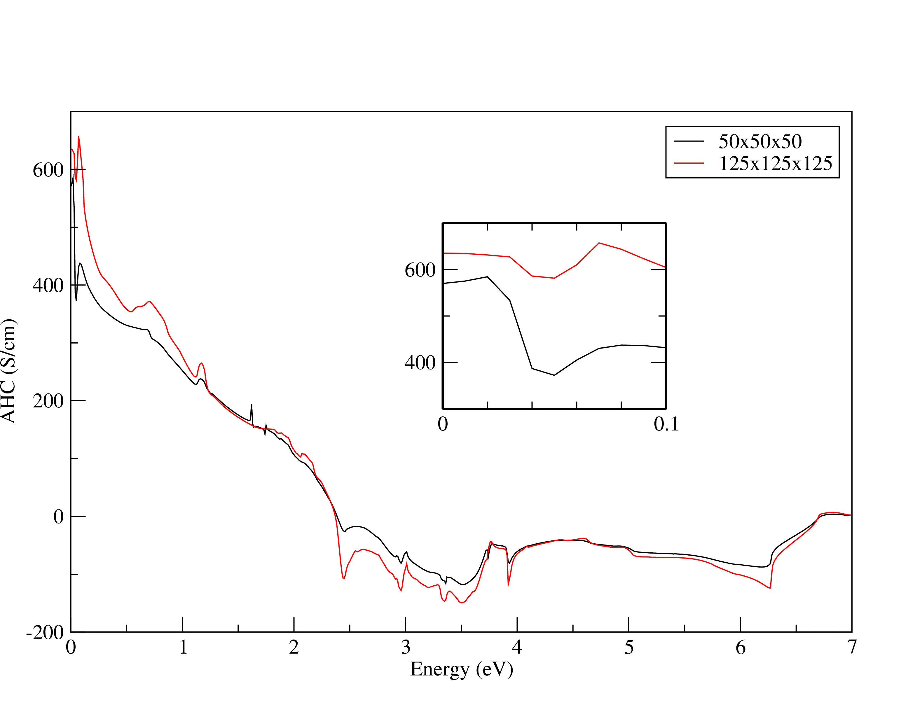
The DC AHC calculated earlier corresponds to \(\sigma_{xy}\) in the limit \(\omega \rightarrow 0\). At finite frequency \(\sigma_{xy} = -\sigma_{yx}\) acquires an imaginary part which describes magnetic circular dichroism (MCD). Compute the complex optical conductivity for \(\hbar\omega\) up to \(7\) eV.

The plot for the ac AHC is shown in Figure 4.

Plot of the real part of the complex optical conductivity with a \(50\times50\times50\) \(k\)-point mesh (black) and \(125\times125\times125\) \(k\)-point mesh (red). The inset is a magnification of the region [0-0.1] eV.

Compare the \(\omega \rightarrow 0\) limit of \(\sigma_{xy}\) with the result obtained earlier by integrating the Berry curvature.

The result obtained by integrating the Berry curvature is 729.83 \((\Omega \mathrm{cm})^{-1}\) and the \(\omega \rightarrow 0\) limit of the complex optical conductivity is \(669.37\) \((\Omega \mathrm{cm})^{-1}\).

Plot the MCD spectrum.

The plot of the magnetic circular dichroism is shown in Figure 5.

The magnetic circular dichroism from interpolation of the Kubo-Greenwood formula.

Further ideas

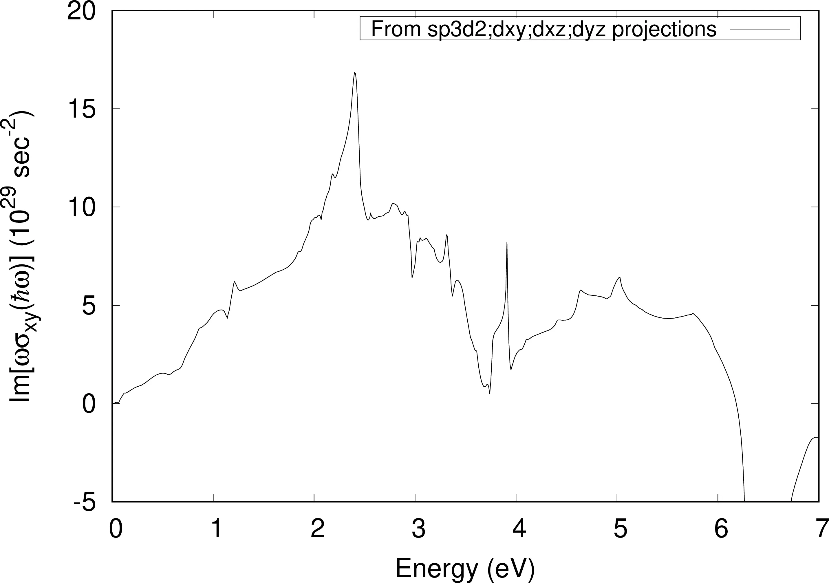
Recompute the AHC and optical spectra of bcc Fe using projected s, p, and d-type Wannier functions instead of the hybridrised MLWFs (see Example 8), and compare the results.

First we have to modify the projection block in the input file Fe.win as did in Tutorial solution 8

Input file

begin projections
Fe:s;p;d
end projections

Then we need to re-do points 3,4 and 6.

Below there is the extract from the output file Fe.wpout. The result obtained from \(s,p\) and \(d\) projections for the \(z\) component, i.e. \(\sigma_{xy}\), of the AHC is exactly the same as the one obtained from \(sp_3d_2,d_{xy},d_{xz}\), and \(d_{yz}\) projections. Plot of AHC and MCD are shown in Figure 6.

With adaptive refinement

 Properties calculated in module  b e r r y
 ------------------------------------------

   * Anomalous Hall conductivity

 Regular interpolation grid: 25 25 25
   Adaptive refinement grid: 5 5 5
       Refinement threshold: Berry curvature >100.00 bohr^2
  Points triggering refinement:   42( 0.27%)

 Fermi energy (ev):   12.6283

 AHC (S/cm)       x          y          z
 ==========
 J0 term :      0.0006    -0.0006    -2.9033
 J1 term :      0.0032    -0.0032    10.0566
 J2 term :      2.4564    -2.4564   567.1417
 -------------------------------------------
 Total   :      2.4602    -2.4602   574.2950

Left panel: Anomalous Hall conductivity. Right panel: Magnetic circular dichroism for \(\hbar\omega\) up to \(7\) eV, starting from \(s;p;d\) initial projections.

---

1. Yugui Yao, Leonard Kleinman, A. H. MacDonald, Jairo Sinova, T. Jungwirth, Ding-sheng Wang, Enge Wang, and Qian Niu. First principles calculation of anomalous hall conductivity in ferromagnetic bcc fe. Phys. Rev. Lett., 92:037204, 2004. ↩↩↩↩

2. Xinjie Wang, Jonathan R. Yates, Ivo Souza, and David Vanderbilt. Ab initio calculation of the anomalous hall conductivity by wannier interpolation. Phys. Rev. B, 74:195118, 2006. ↩↩↩↩

3. M. G. Lopez, David Vanderbilt, T. Thonhauser, and Ivo Souza. Wannier-based calculation of the orbital magnetization in crystals. Phys. Rev. B, 85:014435, 2012. ↩