32: Tungsten — SCDM parameters from projectability¶

Outline: Compute the Wannier interpolated band structure of tungsten (W) using the SCDM method to calculate the initial guess (see Tutorial 27 for more details). The free parameters in the SCDM method, i.e., \(\mu\) and \(\sigma\), are obtained by fitting a complementary error function to the projectabilities. The number of MLWFs is given by the number of pseudo-atomic orbitals (PAOs) in the pseudopotential, \(21\) in this case. All the steps shown in this tutorial have been automated in the AiiDA¹ workflow that can be downloaded from the MaterialsCloud website².
Directory: tutorials/tutorial32/ Files can be downloaded from here
Input files
- W.scf The pwscf input file for ground state calculation
- W.nscf The pwscf input file to obtain Bloch states on a uniform grid
- W.pw2wan The input file for pw2wannier90
- W.proj The input file for projwfc
- generate_weights.sh The bash script to extract the projectabilities from the output of projwfc
- W.win The wannier90 input file

Run pwscf to obtain the ground state of tungsten
Terminal
```
pw.x -in W.scf > scf.out
```
Run pwscf to obtain the Bloch states on a \(10\times10\times10\) uniform \(k\)-point grid
Terminal
```
pw.x -in W.nscf > nscf.out
```
Run wannier90 to generate a list of the required overlaps (written into the W.nnkp file)
Terminal
```
wannier90.x -pp W
```
Run projwfc to compute the projectabilities of the Bloch states onto the Bloch sums obtained from the PAOs in the pseudopotential
Terminal
```
projwfc.x -in W.proj > proj.out
```
Run generate_weights to extract the projectabilitites from proj.out in a format suitable to be read by Xmgrace or gnuplot
Terminal
```
./generate_weights.sh
```
Plot the projectabilities and fit the data with the complementary error function

\[ f(\epsilon;\mu,\sigma) = \frac{1}{2} \mathrm{erfc}(-\frac{\mu - \epsilon}{\sigma}). \]

We are going to use Xmgrace to plot the projectabilities and perform the fitting. Open Xmgrace
Terminal
```
xmgrace
```
To Import the p_vs_e.dat file, click on Data from the top bar and then Import -> ASCII.... At this point a new window Grace: Read sets should pop up. Select p_vs_e.dat in the Files section, click Ok at the bottom and close the window. You should now be able to see a quite noisy function that is bounded between 1 and 0. You can modify the appearance of the plot by clicking on Plot in the top bar and then Set appearance.... In the Main section of the pop-up window change the symbol type from None to Circle. Change the line type from straight to none, since the lines added by default by Xmgrace are not meaningful. For the fitting, go to Data -> Transformations -> Non-linear curve fitting. In this window, select the source from the Set box and in the Formula box insert the following
Input file
```
y = 0.5 * erfc( ( x - A0 ) / A1 )
```
Select 2 as number of parameters, give 40 as initial condition for A0 and 7 for A1. Click Apply. A new window should pop up with the stats of the fitting. In particular you should find a Correlation coefficient of 0.96 and a value of \(39.9756\) for A0 and \(6.6529\) for A1. These are the value of \(\mu_{fit}\) and \(\sigma_{fit}\) we are going to use for the SCDM method. In particular, \(\mu_{SCDM} = \mu_{fit} - 3\sigma_{fit} = 20.0169\) eV and \(\sigma_{SCDM} = \sigma_{fit} = 6.6529\) eV. The motivation for this specific choice of \(\mu_{fit}\) and \(\sigma_{fit}\) may be found in Ref. ³, where the authors also show validation of this approach on a dataset of 200 materials. You should now see the fitting function, as well as the projectabilities, in the graph below.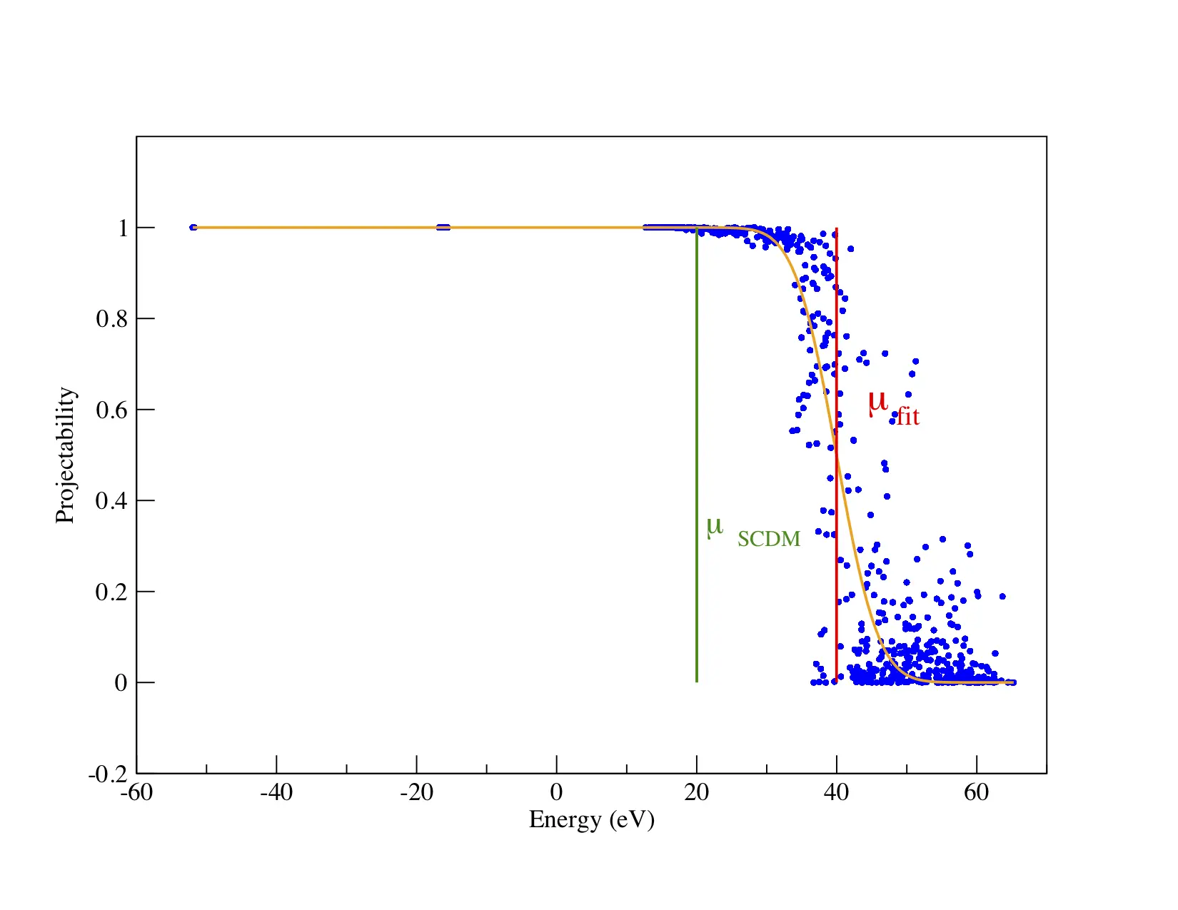

Each blue dot represents the projectability as defined in Eq. (22) of Ref. ³ of the state \(\vert n\mathbf{k} \rangle\) as a function of the corresponding energy \(\epsilon_{n\mathbf{k}}\) for tungsten. The yellow line shows the fitted complementary error function. The vertical red line represents the value of \(\sigma_{fit}\) while the vertical green line represents the optimal value of \(\mu_{SCDM}\), i.e. \(\mu_{SCDM} = \mu_{fit} - 3\sigma_{fit}\).

Open W.pw2wan and append the following lines

Input file

scdm_entanglement = erfc

scdm_mu = 20.0169

scdm_proj = .true.

scdm_sigma = 6.6529

Run pw2wannier90 to compute the overlaps between Bloch states and the projections for the starting guess (written in the W.mmn and W.amn files)
Terminal
```
pw2wannier90.x -in W.pw2wan > pw2wan.out
```
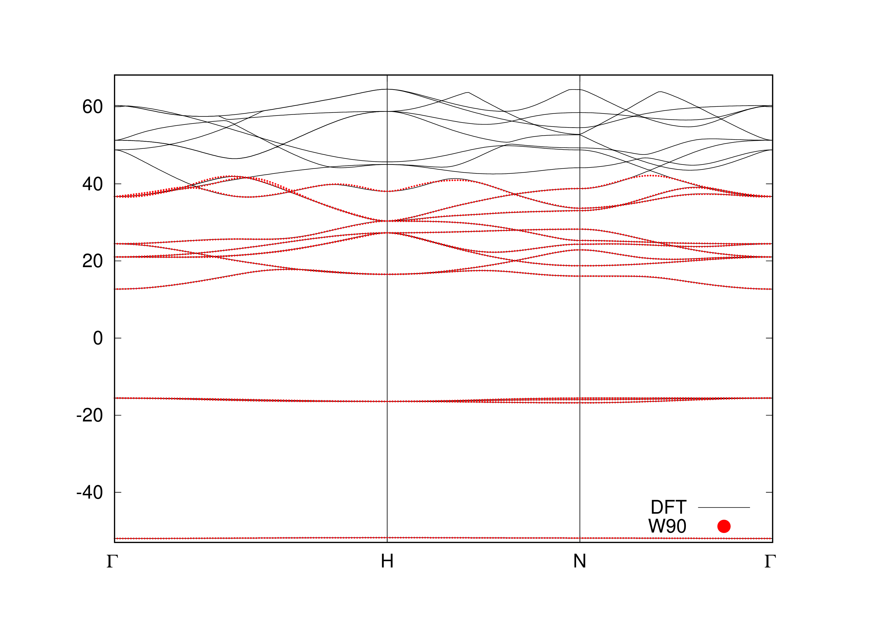
Run wannier90 to obtain the interpolated bandstructure (see the band structure plot).
Terminal
```
wannier90.x W
```
Please cite Ref. ³ in any publication employing the procedure outlined in this tutorial to obtain \(\mu\) and \(\sigma\).

Image title — Band structure of tungsten on the Γ-H-N-Γ path from DFT calculations (solid black) and Wannier interpolation using the SCDM method to construct the initial guess (red dots).

Giovanni Pizzi, Andrea Cepellotti, Riccardo Sabatini, Nicola Marzari, and Boris Kozinsky. Aiida: automated interactive infrastructure and database for computational science. Computational Materials Science, 111:218 – 230, 2016. ↩
V. Vitale, G. Pizzi, A. Marrazzo, J. R. Yates, N. Marzari, and A. A. Mostofi. Automated high-throughput wannierisation. Materials Cloud Archive, 2019. doi:\href http://doi.org/10.24435/materialscloud:2019.0044/v210.24435/materialscloud:2019.0044/v2. ↩
Valerio Vitale, Giovanni Pizzi, Antimo Marrazzo, Jonathan Yates, Nicola Marzari, and Arash Mostofi. Automated high-throughput wannierisation. 2019. arXiv:1909.00433. ↩↩↩