33: Monolayer BC\(_2\)N — \(k\cdot p\) expansion coefficients
-
Outline: Calculate \(k\cdot p\) expansion coefficients monolayer BC\(_2\)N using quasi-degenerate (Löwdin) perturbation theory. In preparation for this example it may be useful to read Ref. 1
-
Directory:
tutorial/tutorial33/Files can be downloaded from here -
Input files:
-
bc2n.scfThepwscfinput file for ground state calculation -
bc2n.nscfThepwscfinput file to obtain Bloch states on a uniform grid -
bc2n.pw2wanThe input file forpw2wannier90 -
bc2n.winThewannier90andpostw90input file
-
-
Run
pwscfto obtain the ground state -
Run
pwscfto obtain the ground state -
Run
Wannier90to generate a list of the required overlaps (written into thebc2n.nnkpfile) -
Run
pw2wannier90to compute:- The overlaps \(\langle u_{n\bf{k}}|u_{n\bf{k+b}}\rangle\)
between spinor Bloch states (written in the
bc2n.mmnfile) - The projections for the starting guess (written in the
bc2n.amnfile)
- The overlaps \(\langle u_{n\bf{k}}|u_{n\bf{k+b}}\rangle\)
between spinor Bloch states (written in the
-
Run
wannier90to compute MLWFs -
Run
postw90to compute expansion coefficients
Expansion coefficients
For computing \(k\cdot p\) expansion coefficients as given by quasi-degenerate (Löwdin) perturbation theory, set
Select the k-point around which the expansion coefficients will be computed, e.g., the S point
Set number of bands that should be taken into account for the \(k\cdot p\) expansion, as well as their band indexes within the Wannier basis
Since no k-space integral is needed, set
Although not used, we also need to input the value of the Fermi level in eV
On output, the program generates three files, namely
SEED-kdotp_0.dat, SEED-kdotp_1.dat and SEED-kdotp_2.dat, which
correspond to the zeroth, first and second order expansion coefficients,
respectively. The dimension of the matrix contained in each file is
\(3^{l}\times N^{2}\), where \(N\) is the number of bands set by kdotp_num_bands,
and \(l\) is the order of the expansion term (currently \(l=0,1\) or \(2\)).
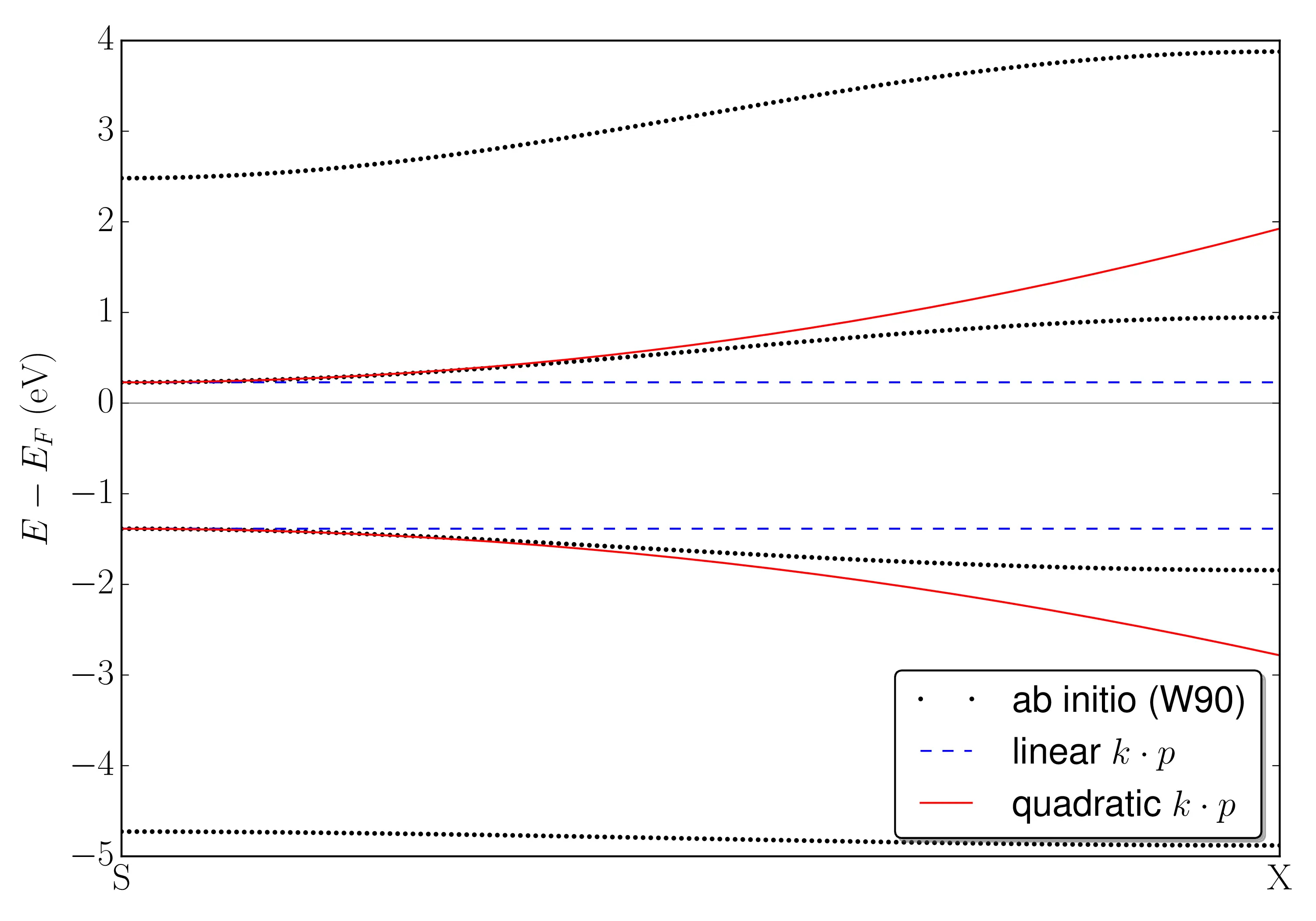
These coefficients can be used, among other things, to compute the
energy dispersion of the bands of interest around the chosen
k-point. The \(k\cdot p\) band dispersion can be computed and plotted
along \(k_x\) (from S to X) using python and the file kdotp_plot.py
provided in the example folder
For comparison, the exact band structure calculated usingWannier90
(file bc2n_band.dat, generated automatically) is also plotted along
(see the band dispersion plot).
-
Julen Ibañez-Azpiroz, Fernando de Juan, and Ivo Souza. Quantitative analysis of two-band \(k\cdot p\) models describing the shift-current photoconductivity. ArXiv e-prints, 2019. URL: http://arxiv.org/abs/1910.06172, arXiv:1910.06172. ↩