4: Copper — Fermi surface, orbital character of energy bands¶

Outline: Obtain MLWFs to describe the states around the Fermi-level in copper
Generation Details: From pwscf, using ultrasoft pseudopotentials ¹ and a
4\(\times\)4\(\times\)4 k-point grid. Starting guess: five atom-centred d orbitals, and two s orbitals centred on one of each of the two tetrahedral interstices.
Directory: tutorials/tutorial04/ Files can be downloaded from here
Input Files
- copper.win The master input file
- copper.mmn The overlap matrices \(\mathbf{M}^{(\mathbf{k},\mathbf{b})}\)
- copper.amn Projection \(\mathbf{A}^{(\mathbf{k})}\) of the Bloch states onto a set of trial localised orbitals
- copper.eig The Bloch eigenvalues at each k-point
Run wannier90 to minimise the MLWFs spread
Terminal
```
wannier90.x copper
```
Inspect the output file copper.wout.
Plot the Fermi surface, it should look familiar! The Fermi energy is at 12.2103 eV.

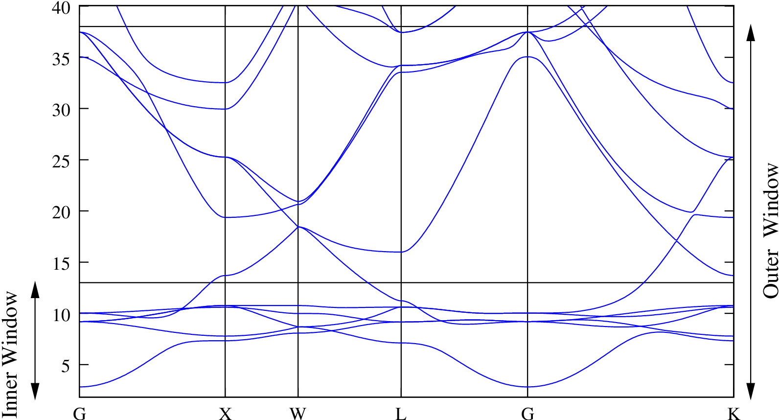
Plot the interpolated bandstructure. A suitable path in k-space is

Input file

 begin kpoint_path
 G 0.00 0.00 0.00 X 0.50 0.50 0.00
 X 0.50 0.50 0.00 W 0.50 0.75 0.25
 W 0.50 0.75 0.25 L 0.00 0.50 0.00
 L 0.00 0.50 0.00 G 0.00 0.00 0.00
 G 0.00 0.00 0.00 K 0.00 0.50 -0.50
 end kpoint_path

Plot the contribution of the interstitial WF to the bandstructure. Add the following keyword to copper.win
Input file
```
bands_plot_project = 6,7
```
The resulting file copper_band_proj.gnu can be opened with gnuplot. Red lines correspond to a large contribution from the interstitial WF (blue line are a small contribution; ie a large \(d\) contribution).

Investigate the effect of the outer and inner energy window on the interpolated bands.

Image title — Bandstructure of copper showing the position of the outer and inner energy windows.

D. Vanderbilt. Phys. Rev. B, 41:7892, 1990. ↩